From Molecules to Matrices and back again 🧬 - Part 2: Why the Mean Wins

The Humbling Reality of Perturbation Prediction in the Virtual Cell Challenge

Part 1 covered the biology: DNA, RNA, gene expression, how single-cell RNA-seq produces sparse matrices. Now we predict perturbation effects and learn why the simplest baseline is so hard to beat. I set myself for the challenge to gauge the upper bound of what’s achievable using only the provided data. No foundation models, no protein networks, no external knowledge. Just 221K cells and standard ML. Spoiler: the ceiling is low.*

What We’re Trying to Predict

The Virtual Cell Challenge asks us to predict how cells respond to genetic perturbations. Given that we knock out (silence) a gene using CRISPR, what will the cell’s expression profile look like?

The Data:
- 221,273 cells × 18,080 genes
- 151 unique CRISPR knockouts (perturbations)
- ~38,000 control cells (non-targeting guides)
- ~52% sparsity (most genes aren’t expressed in most cells)

The Zero-Shot Problem

Here’s the catch: we must predict effects for genes we’ve never seen during training.

The challenge splits genes (not cells) into train and test sets. From the 150 provided target genes, I trained on 120 knockout genes, tested on 30 completely different knockouts. We can’t memorize “when you knock out Gene X, here’s what happens.” We need to learn something transferable about how perturbations affect cells.

Train Set: 120 genes → 178,256 cells
Test Set: 30 genes → 43,017 cells (COMPLETELY UNSEEN)

This is fundamentally different from most ML problems where train and test come from the same distribution. Here, the test distribution is deliberately different.

---

The Metrics

The official challenge uses three metrics: Differential Expression Score (DES), Perturbation Discrimination Score (PDS), and MAE, with the final leaderboard score calculated as scaled improvement over a cell-mean baseline.

Running the full evaluation suite is computationally expensive on my computer. For rapid iteration, I used cell-eval with minimal settings to compare methods quickly. These metrics from the cell-eval capture similar concepts to the official ones:

Pearson Delta

Correlation between predicted perturbation effect and actual perturbation effect:

For each perturbation:
  delta_pred = pred_perturbed_mean - pred_control_mean
  delta_real = real_perturbed_mean - real_control_mean
  pearson_delta = correlation(delta_pred, delta_real)

Why it matters: Raw expression is dominated by housekeeping genes that don’t change much. Pearson Delta measures whether you’re capturing the direction of changes: which genes go up, which go down. Not part of official scoring, but useful for quick iteration.

Overlap@N (Related to DES)

Overlap between predicted and actual differentially expressed genes:

1. Filter to significant genes (FDR < 0.05)
2. Sort by absolute log2 fold change
3. overlap = |predicted_sig ∩ actual_sig| / |actual_sig|

Why it matters: Similar concept to the official DES metric. Biologists care about correctly identifying which genes are significantly affected. The metric uses statistical significance (FDR threshold) plus fold change ranking.

Discrimination Score (L1 Distance) - PDS

Can we tell different perturbations apart based on their predicted profiles?

For each predicted perturbation p:
  1. Compute L1 distance from pred_delta[p] to ALL real_deltas
  2. Rank real perturbations by distance (ascending)
  3. Find rank of the correct perturbation
  4. Score = 1 - (rank / n_perturbations)
  
Score of 1.0 = correct perturbation has lowest distance
Target gene excluded from distance calculation

Why it matters: This is essentially the official Perturbation Discrimination Score (PDS). Does our prediction look most similar to the correct perturbation? A random baseline scores ~0.5.

MAE (Mean Absolute Error)

Standard reconstruction error on pseudobulk expression:

For each perturbation:
  pred_mean = mean expression across predicted cells
  real_mean = mean expression across actual cells
  MAE = mean(|pred_mean - real_mean|) across all genes

Why it matters: Captures overall prediction accuracy across all genes, including those that don’t change. Same as the official MAE metric.

Quick Reference

Pearson Delta : Direction of changes : Higher → better (not in official scoring) Overlap@N : DE gene overlap : Higher → better (approximates DES)
Discrimination (L1) : Perturbation specificity : 1.0 = perfect (PDS)
MAE : Absolute error : Lower → better (official metric)

---

The “Boring UMAP” Revelation

Before building models, I looked at the data.

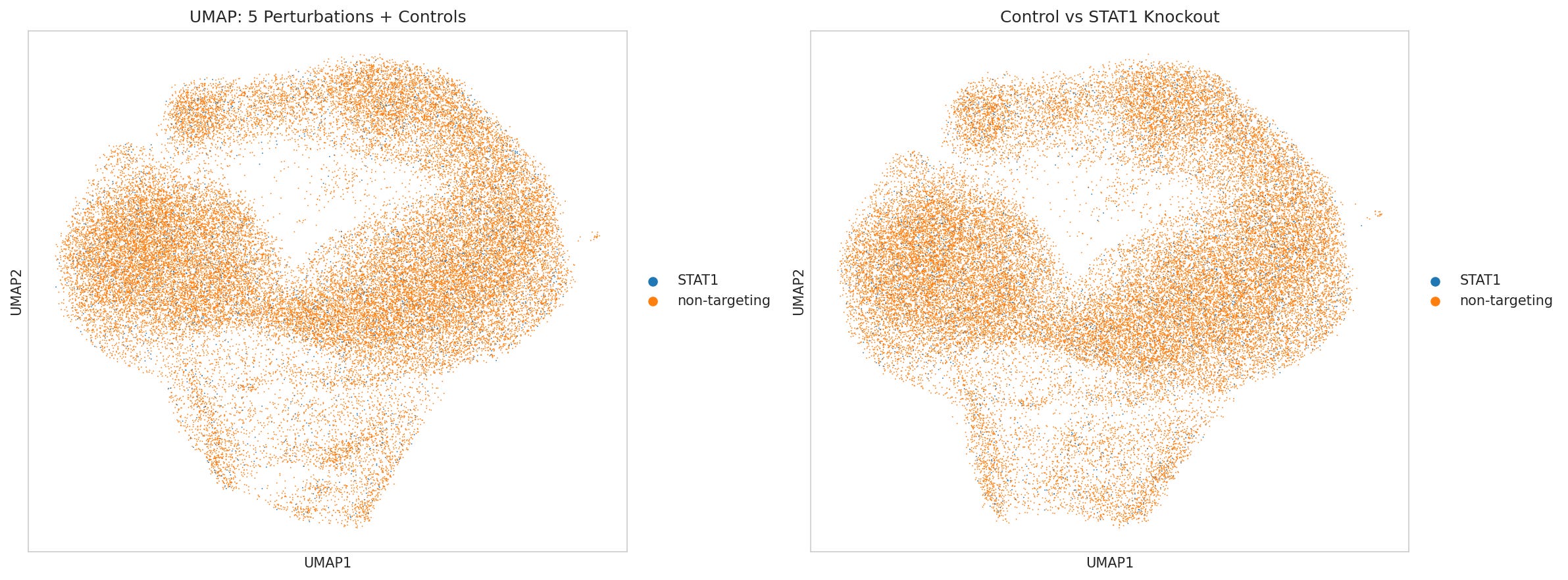
What I expected: Different knockouts → different cell states → distinct UMAP clusters.

What I got: A blob. Literally one giant blob with control and perturbed cells completely overlapping. My first thought: “Did I mess up the normalization?”

Figure 1. Control vs. Purturbed mean distribution comparison (Left). Distribution of perturbation delta from Control mean (Right)

Figure 2. Heatmap of knockdown effect of target gene on top 100 variable genes

Figure 3. UMAP of top 5 perturbations and Control hugely overlapping.

The Investigation

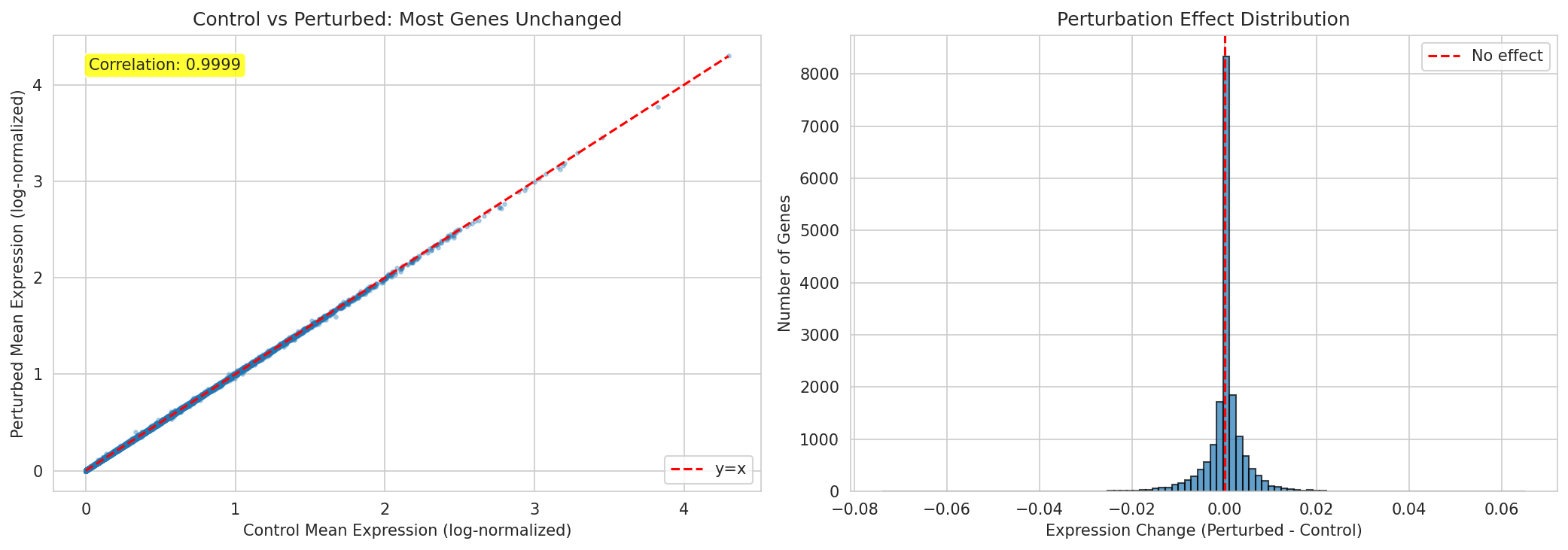
Check 1: Control vs. Perturbation Correlation

control_mean = adata[control_cells].X.mean(axis=0)
perturbed_mean = adata[perturbed_cells].X.mean(axis=0)
correlation = np.corrcoef(control_mean, perturbed_mean)[0,1]
# Result: 0.98+  Almost identical!

Check 2: How Many Genes Actually Change?

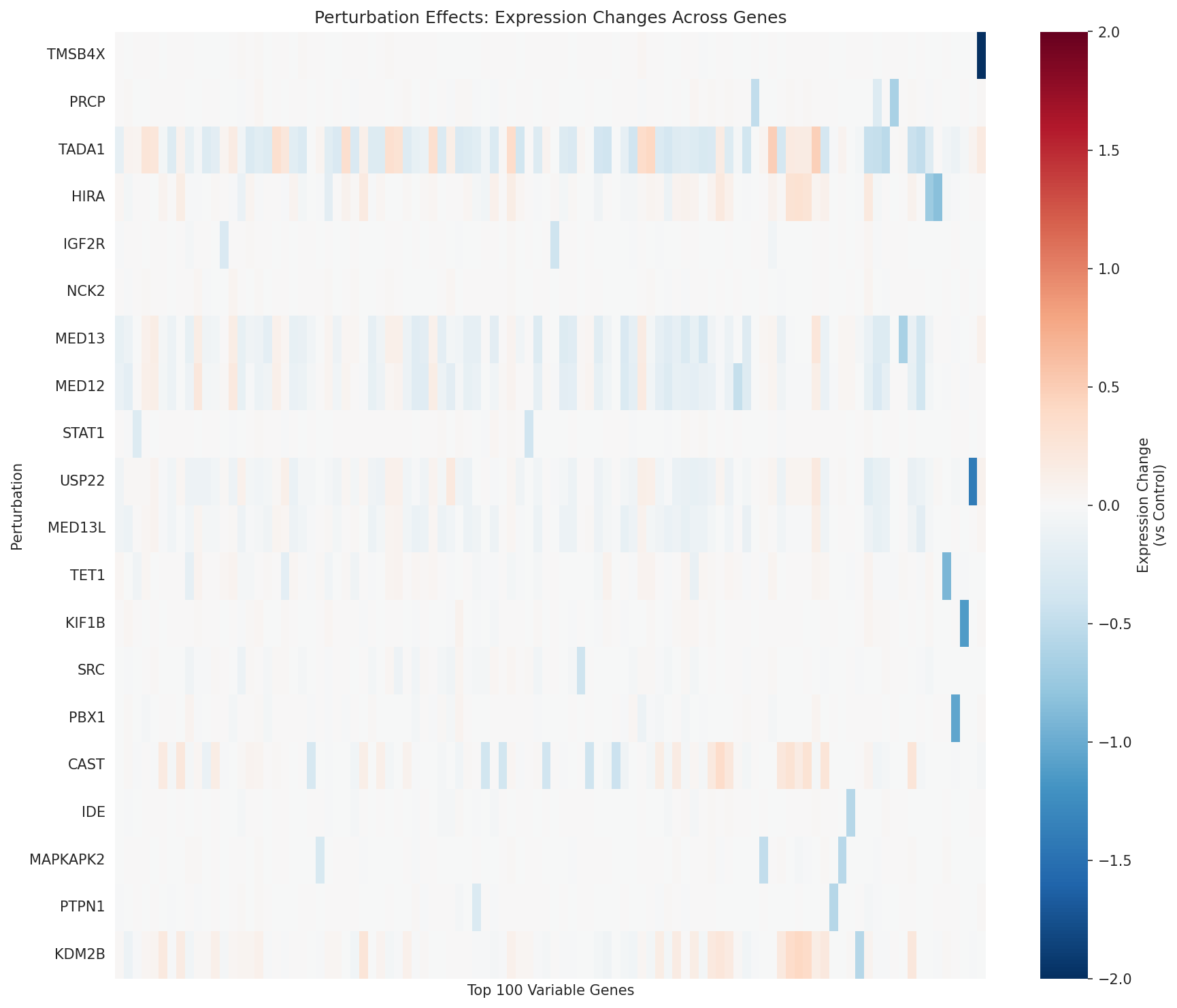
Genes with |change| > 0.5:  ~500 / 18,080  (2.8%)
Genes with |change| < 0.25: ~16,000 / 18,080 (88%)

The Realization

The UMAP isn’t broken. This IS the biology.

Knocking out one gene doesn’t transform a cell into something completely different. It causes subtle ripples in a handful of downstream genes while 97% stay essentially the same. The cell is still the same cell type, doing mostly the same things, just with one pathway disrupted.

We’re not trying to predict 18,080 genes. We’re trying to predict the ~3% that actually change. But we don’t know which 3% in advance.

---

The Cell Mean Baseline (Why It’s Hard to Beat)

class CellMeanBaseline:
    def fit(self, adata_train):
        perturbed_mask = adata_train.obs['target_gene'] != 'non-targeting'
        self.context_mean = adata_train[perturbed_mask].X.mean(axis=0)
    
    def predict(self, n_cells):
        return [self.context_mean] * n_cells

No neural networks. No embeddings. Just predict the average perturbed cell for every prediction.

Cell Mean Baseline Performance:
├── Pearson Delta:    0.1882  ← Our target to beat!
├── Overlap@N:        0.0931
├── Discrimination:   0.5167
├── MSE:              0.001392
└── MAE:              0.014075

Why Does This Work So Well?

1. Most Genes Don’t Change (97% “Free”)

If 97% of genes are essentially unchanged by any perturbation, then predicting “average perturbed cell” is already 97% correct for those genes.

2. Perturbation Effects Are Subtle

The few genes that DO change don’t change by much. The delta between control and perturbed is small compared to the baseline expression level. So even a blunt average captures the general direction.

3. Cells Are Similar to Their Mean

Within any perturbation group, individual cells correlate 95%+ with their group mean. This is biological reality: cells in the same condition are doing similar things.

          Control Mean  vs.  Perturbed Mean
          ────────────       ──────────────
Gene A:       5.2                5.3        (+0.1)
Gene B:       0.8                0.7        (-0.1)  
Gene C:       3.1                3.0        (-0.1)
Gene D:       0.0                0.1        (+0.1)  ← The signal!
...
Gene 18000:   2.1                2.1        (0.0)

The context mean captures the “typical perturbed cell” profile. Since all perturbations share 97% of their profile, it’s a surprisingly good guess.

To Beat the Mean

We need to:

1. Identify WHICH genes will change for THIS perturbation

2. Predict the DIRECTION and MAGNITUDE of change

3. Do this for perturbations you’ve NEVER SEEN

And you only have ~1,200 cells per perturbation to learn from. Compare that to ImageNet with millions of images per class!

---

My Failed Experiments

I had been thinking about how diffusion models could help here but with low data, I really wanted to jump straight to VAEs for quick experiments. Neural nets should simply work. Right?

Attempt 1: VAE with Correlation Transfer

The Idea:

• Train a VAE to reconstruct cell expression

• Learn perturbation embeddings that capture knockout effects

• For unseen genes, find correlated genes in training and “borrow” their embeddings

Architecture:

[Expression (18080d)] + [Pert Embedding (32d)] 
    → Encoder → Latent Z (64d)
    → Decoder → [Predicted Expression (18080d)]

The Result:

VAE + Correlation Transfer:
├── Pearson Delta:    0.0273  ← 85% WORSE than mean!
├── Overlap@N:        0.0766
└── Discrimination:   0.5100

What Went Wrong:

Expression correlation ≠ functional similarity. Two genes might co-express (high correlation) but have completely different knockout effects.

The VAE is optimizing for reconstruction, not for capturing perturbation-specific signals. It learns to predict “average cell” because that minimizes reconstruction error.

Attempt 2: VAE with Learned Gene Embeddings

The Idea:

• Instead of using expression correlation, learn gene embeddings during training

• Use contrastive learning (alignment + triplet loss) to make similar genes cluster

• Transfer to unseen genes via embedding similarity

Architecture:

Same VAE + Gene Embedding Layer (18080 × 16d)
+ Alignment Loss: similar perts → similar embeddings
+ Triplet Loss: separate different perturbations

Training:

VAE w/ Gene Embeddings: 9,674,112 parameters
Training for 300 epochs...
  Epoch 100: Loss = 0.0241, Align = 0.0633, Triplet = 0.2634
  Epoch 200: Loss = 0.0241, Align = 0.0630, Triplet = 0.2647
  Epoch 300: Loss = 0.0240, Align = 0.0627, Triplet = 0.2625

The Result:

VAE + Learned Embeddings:
├── Pearson Delta:    0.0226  ← 88% WORSE than mean!
├── Overlap@N:        0.0773
└── Discrimination:   0.5144

What Went Wrong:

Same fundamental issue. The VAE is still optimizing to reconstruct the input. The gene embeddings learn generic patterns, not perturbation-specific signals. 300 epochs doesn’t change the fact that predicting “average” is statistically optimal for reconstruction loss.

Attempt 3: Residual Learning

The Insight: Stop trying to predict absolute expression. Predict the change from the context mean baseline:

# Instead of: model(cell) → expression
# We Do:      model(cell) → delta
#             prediction = context_mean + delta
# 
# where context_mean = mean of all perturbed training cells (our 0.188 baseline!)

This forces the model to focus on what actually differs between perturbations, rather than reconstructing the 97% that stays the same. This is like finding remaining value to capture.

Architecture:

Residual VAE: 9,674,080 parameters
Training on DELTAS for 300 epochs...
  Epoch 100: Loss = 0.2214, MeanDelta = 0.0466
  Epoch 200: Loss = 0.2198, MeanDelta = 0.0439
  Epoch 300: Loss = 0.2200, MeanDelta = 0.0436

The Result:

VAE Residual:
├── Pearson Delta:    0.0781  ← Better! But still 58% worse than mean
├── Overlap@N:        0.0902
└── Discrimination:   0.5133

Progress! But still not beating the baseline. The model learns some structure in the deltas but the signal is weak.

Attempt 4: Numerai-Style Neutralization

The Idea (from quantitative finance):

Building on residual learning, I noticed the predicted deltas still contained common patterns across all perturbations, shared responses like stress signatures or cell cycle effects. What if these common patterns are noise that doesn’t generalize to unseen genes?

This reminded me of some early Numerai financial models I used to build. Numerai doesn’t just reward raw accuracy (Correlation), it rewards MMC (Meta Model Contribution): how much unique signal your model adds beyond what the ensemble already captures.

The intuition: if everyone predicts the same pattern even if it’s residual, that pattern is already “priced in.” Value comes from orthogonal predictions that capture something the consensus misses.

Inspired by that, translated to perturbation prediction:

• The “meta-model” is the context mean baseline

• Common delta patterns (shared across perturbations) are the “consensus”

• Unique signal = perturbation-specific effects that differ from common responses

Implementation:

# 1. Compute per-perturbation mean deltas from context mean
for pert in perturbations:
    delta[pert] = perturbed_mean[pert] - context_mean

# 2. Stack into matrix and extract common factors via SVD
delta_matrix = stack([delta[p] for p in perturbations])  # shape: (n_perts, n_genes)
U, S, Vt = SVD(delta_matrix)
common_factors = Vt[:k].T  # top k principal components

# 3. For each prediction, remove projection onto common factors (orthogonalize)
def neutralize(delta, factors):
    projection = factors @ (factors.T @ delta)
    return delta - projection

The idea: by removing patterns shared across all perturbations, we isolate signals specific to individual knockouts, the actual biology we care about.

The Result:

VAE Residual (Neutralized):
├── Pearson Delta:    0.1090  ← Getting closer!
├── Overlap@N:        0.0874
└── Discrimination:   0.5167

Progress! Neutralization helps by removing common artifacts. But we’re still 42% below the mean.

Attempt 5: Delta Library

The Idea: Forget the neural network decoder. Store the mean delta for each training perturbation, do nearest-neighbor lookup:

# Training: store mean delta per perturbation
self.delta_library = {
    'TP53': mean_delta_for_TP53,
    'BRCA1': mean_delta_for_BRCA1,
    ...
}

# Prediction: find similar genes by embedding, use their deltas
similar_genes = find_nearest_neighbors(unseen_gene_embedding)
predicted_delta = weighted_average([delta_library[g] for g in similar_genes])

The Result:

Delta Library:
├── Pearson Delta:    0.0826  ← Similar to VAE Residual
├── Overlap@N:        0.0921
└── Discrimination:   0.5022

This simple lookup works about as well as the neural network. The bottleneck isn’t the decoder, it’s the transfer mechanism.

After all that work, Not a single method beat the mean.

---

What I Learned

1. Simple Baselines Encode Real Structure

The mean isn’t “dumb.” It captures genuine biological reality:

• Most genes don’t change

• Cells are similar within conditions

• The “average perturbed cell” is a statistically sound prediction

Lesson: Always understand WHY your baseline works before trying to beat it.

2. More Parameters ≠ Better Predictions

Cell Mean:           0 parameters     → Pearson 0.188
VAE + Embeddings:    9.6M parameters → Pearson 0.023

The neural network has 9.6 million parameters and performs 88% worse than storing a single vector.

Lesson: When your signal is weak, adding capacity just overfits to noise.

3. Transfer Learning is the Bottleneck

Every method struggled with unseen genes. The pattern was consistent:

• Works okay on training genes

• Falls apart on test genes

• Expression correlation is a poor proxy for functional similarity

Lesson: The challenge isn’t reconstruction. It’s transfer.

4. Domain Knowledge is the Unlock

What we NEED but don’t have:

Protein networks (STRING) → “Gene A physically interacts with Gene B”
Pathway databases (KEGG) → “These genes are in the same pathway”
Prior perturbation data → “These knockouts have similar effects”
Foundation models → Pre-learned gene relationships from millions of cells

Expression correlation tells us “these genes are co-expressed.” But that’s not the same as “knocking out these genes has similar effects.”

5. The Challenge is the 3%, Not the 97%

Most genes don’t change. The competition is about predicting:

• WHICH genes change

• In WHAT direction

• By HOW MUCH

And doing this for perturbations you’ve never seen.

---

The Path Forward: Foundation Models

• Arc State Model - 270 million cells

• scGPT - 33 million cells

• Geneformer - 30 million cells

These models learn gene relationships from vastly more data than any single experiment. They encode knowledge like:

• Gene X and Gene Y are often perturbed together

• This gene family tends to respond similarly to knockouts

• These pathway members show coordinated changes

This is the external knowledge that pure reconstruction-based learning can’t capture from 221K cells.

---

Key Takeaways

For Data Scientists Entering Computational Biology:

1. Simple baselines encode real structure. The mean captures biology. Understand WHY your baseline works before trying to beat it.

2. More data ≠ better predictions. 221K cells sounds like a lot, but it’s ~1,200 per perturbation. Signal quality matters more than quantity.

3. Domain knowledge is the unlock. Pure ML on biological data has limits. External knowledge (networks, pathways, pre-training) is essential.

4. The challenge is the 3%, not the 97%. Most genes don’t change. The competition is about predicting the handful that do. Metrics like Pearson Δ capture this better than MSE.

The Honest Summary

I spent weeks training neural networks with millions of parameters. The result? 88% worse than storing a single average vector.

But that’s the point. This challenge exists because perturbation prediction is genuinely hard. The mean being hard to beat isn’t a bug, it’s the whole problem statement.

The winning approaches:

Virtual Cell Challenge 2025 Wrap-Up: Winners and Reflections

---

Resources

• Virtual Cell Challenge

• Part 1: Biological Fundamentals

• Arc State Model

• scGPT

• Geneformer

• cell-eval

• LLMs

---

If you’ve found ways to actually beat the mean, I’d love to hear about them. there certainly are some gaps, oversimplifications, please feel free to point them out or expand in the comments.

Thank you for reading, I really appreciate your time!